by David Gracey
This tip is for fellow Excel nerds out there. It will probably be old news for you financial advisors and other folks who work daily with Excel. Regardless of whether you have heard of “Conditional Formatting” or not, this tip is for you. As sad as this sounds, much of my life centers around Excel spreadsheets: computer inventory sheets, monthly bank account summaries and lists of varying types. I’ve used Excel most of my adult life but until recently I had never used Conditional Formatting of cells, so this was new to me.
Let’s say you have a list of some sort and you have several columns of information. At work we keep track of our clients’ computers, when they were purchased and what software runs on them. It is important to know the age of the computers because each year, our clients budget for purchasing new computers. Having this information handy allows us to make informed decisions about who is going to get a new computer this year. Below is the spreadsheet that we use:
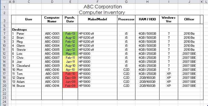
Column E is the date the computer was purchased. I want to show the newest computers in green, older computer in yellow and really old computers in red. This really helps the oldest computers stand out and lets our clients decide when Adam will get that new computer he’s been waiting for. I’ve created a formula behind the scenes that automatically changes the color of the cell based on the age of the computer. If I were to manually fill each cell with the green/yellow/red, then I’d have to adjust it each time I printed out the spreadsheet. A much better way is to use Conditional Formatting and create 3 rules. Here’s how: highlight the cells you want to format, in my example that’s cells E7 thru E20, and click on “Condition Formatting” from the HOME menu bar.
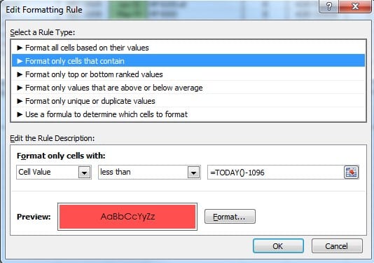
That will bring up a dialog box where you click NEW RULE. In my case I create three rules, one for each color. The tricky part is to know what formula to enter to get the desired results. You can use a cool function, TODAY(), that returns the value of today’s date. When you subtract 1,096 days from today, you get a date 3 years ago. So make the color for that RED by clicking the FORMAT button and choosing a fill color. The result will be a RED cell for any date older than 3 years ago.
Save this rule and create two more rules, one for green and one for yellow. Now every time you open the spreadsheet, the colors will be updated based on the current age of the computers.